How to Improve TSP-Tours Applying the 2-opt Neighborhood

Posted on 27. August 202428. August 2024 by Fabian Leuthold

In this post, we’ll learn how to improve TSP tours using a well known and approved local search improvement heuristic approach. These improvement heuristics start with an initial solution and iteratively improve it until no further improvement is possible, then return the best solution found.

Previously, we discussed how to generate initial solutions for TSP problems. We’ll use the nearest-neighbor construction heuristic to create a starting solution and then enhance it using local search.

How does Local Search work?

Local search relies on two functions: a neighborhood function $N(S)$ and an objective function $f(S)$ .

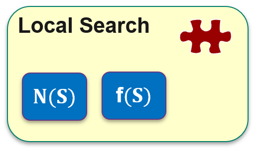
The neighborhood function generates a set of neighboring solutions for a given starting solution, while the objective function provides a value for each (neighboring) solution.

Additionally, we need a meta-heuristic that manages the interaction between the construction and improvement heuristics and guides the solution selection process during local search. This meta-heuristic orchestrates the overall process.

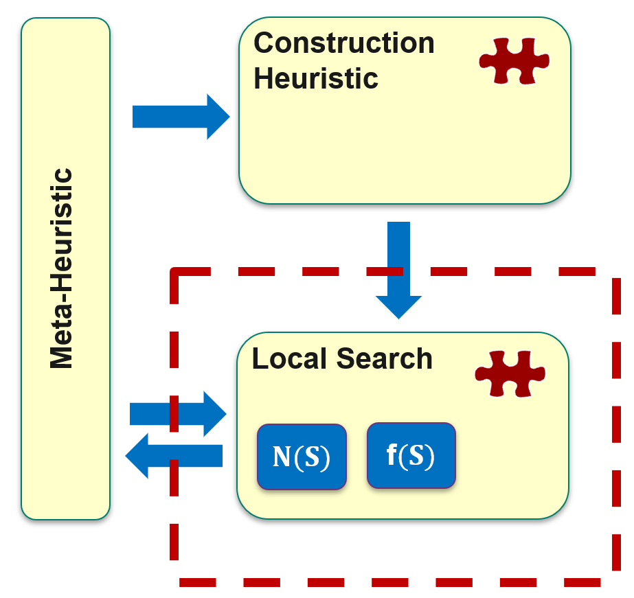
With each candidate solution, the local search provides the corresponding objective function value. The meta-heuristic then uses a specific solution selection method to choose which solution will be the starting point for the next local search.

Two Local Search Flavours

The meta-heuristic repeatedly triggers local searches until no further improvement is possible. In each iteration, it selects the next solution to start the local search. If all neighbors are evaluated and the best one is chosen, it’s called the Best Improvement method. Alternatively, if the meta-heuristic starts a new local search immediately after finding any better candidate solution, it’s known as the First Improvement method. We’ll apply the best improvement solution selection method here.

The 2-opt Neighborhood

Looking at the solutions from the nearest neighbor construction heuristic in this post, we notice that the line segments of some tour sections cross each other. Such solutions are definitely not optimal if the cost function is based on Euclidean distances. For example, let’s take a look at the solution from the nearest neighbor construction heuristic for the berlin52 problem instance, when triggered with start node 1:

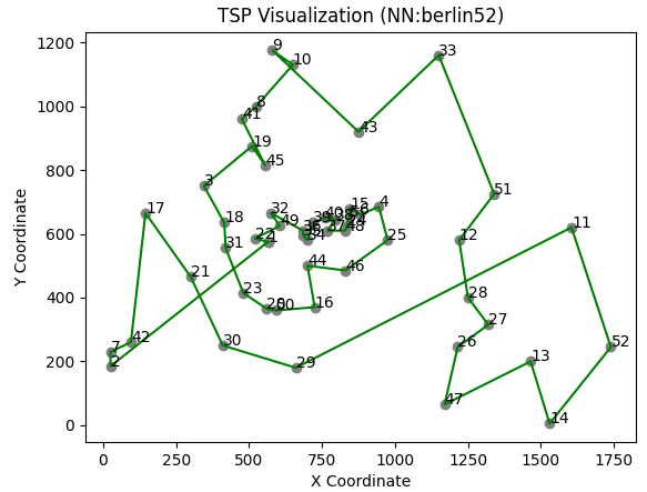
*Solution of berlin52 with NN-construction heuristic, starting at node (1)*

The 2-opt neighborhood is a neighborhood designed to address this issue. It involves selecting (any) two edges in a tour, removing them, and reconnecting the tour in the opposite order. This creates a new, often shorter tour. It’s effective for finding neighboring solutions because it allows for simple, yet powerful, improvements to the current tour by eliminating crossings and reducing the total distance.

Since it would be too ‘expensive’ to first determine which line segments have intersections, it’s easier to evaluate all possible 2-opt neighbors.

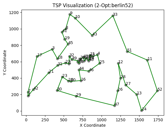
This solution is still 7% longer than the optimal solution, but it’s already 11% better than the initial solution from the NN construction heuristic.

How to Apply a 2-opt Swap

The 2-opt swap can be simplified as follows:

Select 2 nodes
Swap the order of all the nodes in between, including the selected nodes

Example: S = [1, 2, 3, 4, 5, 6]
Selected Nodes: 2, 3, 4, 5
Swapped Nodes: 5, 4, 3, 2

Resulting Tour: S’ = [1, 5, 4, 3, 2, 6]

Bringing it All together

We can now implement our local search using the 2-opt neighborhood. With the best improvement approach, we’ll evaluate the entire 2-opt neighborhood in each iteration and choose the best solution. When no further improvements are possible, the search ends and we return the best solution:

def tsp_local_search(nodes, initial_solution):
    # Initialize the best solution and its distance
    best_solution = initial_solution
    best_distance = total_tour_distance(best_solution, nodes)
    improvement = True

    # Continue searching for improvements while possible
    while improvement:
        improvement = False
        for i in range(1, len(best_solution) - 1):
            for k in range(i + 1, len(best_solution)):
                # Generate a new solution by performing a 2-opt swap
                new_solution = two_opt_swap(best_solution, i, k)
                # Calculate the distance of the new solution
                new_distance = total_tour_distance(new_solution, nodes)
                # Check if the new solution is better
                if new_distance < best_distance:
                    best_solution = new_solution
                    best_distance = new_distance
                    improvement = True

    return best_solution, best_distance

Based on the above considerations for the 2-opt swap, we can implement the two_opt_swap function as follows:

def two_opt_swap(tour, i, k):
    new_tour = tour[0:i] + tour[i:k + 1][::-1] + tour[k + 1:]
    return new_tour

Next, we need the function to calculate the total tour length. ne straightforward approach is to compute it piece by piece using the Pythagorean theorem:

def total_tour_distance(tour, nodes):
    distance = 0.0
    for i in range(len(tour) - 1):
        distance += calculate_distance(nodes[tour[i]], nodes[tour[i + 1]])
    distance += calculate_distance(nodes[tour[-1]], nodes[tour[0]])  # Return to start
    return distance

Based on the basics from the previous post, we now have a complete script for solving TSP using the NN construction heuristic and improving solutions with 2-Opt local search. See complete source code here.

While construction heuristics are often fast due to their greedy nature, it’s crucial to consider computation speed when implementing improvement heuristics.

Upon closer inspection of our meta-heuristic code, we find that calculating the tour length involves a lot of redundant computations. In an endless loop with nested loops, distances for often the same tour segments are repeatedly calculated. Even though a 2-opt swap only changes the length of two segments, all other segments are recalculated unnecessarily.

A simple solution is memoization, where method calls and return values are cached. A better approach is to focus calculations only on the changing segments and perform delta calculations. This version attempts to improve distance calculations by using delta computations. In addition I added some code for the visualization of TSP solutions. See improved complete source code here.

Validation

To validate our implementation, we can create simple test instances where we know the expected result. A straightforward example would be a starting solution that travels through the corners of a square, where the tour includes crossing diagonals, meaning it contains an intersection of two line segments. We’ll create the following TSP test instance:

NAME: test4
TYPE: TSP
COMMENT: 4 locations on a square with sidelength 20 and left lower edge in (0/0) (Leuthold)
DIMENSION: 4
EDGE_WEIGHT_TYPE: EUC_2D
NODE_COORD_SECTION
1 0 0
2 20 0
3 20 20
4 0 20
EOF

Now, we initiate the local search with the tour [1, 2, 4, 3]:

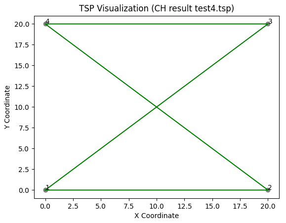
Bad initial solution for our simple test4 TSP instance

Starting the local search with the 2-opt neighborhood on this solution, we expect the intersection to be resolved, resulting in a tour [1, 2, 3, 4] that follows the perimeter of the square.

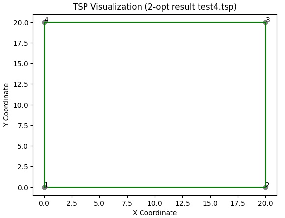
To formally test our expectations for the code, it’s best to encapsulate them in a unit test. This test will check if the local search yields the expected solution, for example, using pytest:

def test_ls_test_1():
    """
    test whether swapped nodes/edges on test4.tsp are detected and solved by 2-opt local search

    :return:
    """
    file_path = './data/test4.tsp'
    nodes = read_tsp_file(file_path)
    tour = [1, 2, 4, 3]
    # plot_tsp_solution(nodes, tour, "CH result test4.tsp")
    tour, dist = tsp_local_search(nodes, tour)
    # plot_tsp_solution(nodes, tour, "2-opt result test4.tsp")
    assert tour == [1, 2, 3, 4], f"Expected tour to be the sequence of 1-8, but got {tour}"
    # make sure, tour distance summary equals to the 4x5 units pieces + 4x5xsqrt(2) units pieces
    assert dist == 80, "Expected distance to be 80, but got other result."

To test heuristic implementations, it’s often helpful to visualize the solutions. With ChatGPT, you can quickly create a method based on a description of the input data. Here’s a function to plot TSP tours:

def plot_tsp_solution(nodes, solution, title):
    # Extract coordinates
    x_coords = [nodes[node][0] for node in solution]
    y_coords = [nodes[node][1] for node in solution]

    # Add the start point to the end to complete the tour
    x_coords.append(nodes[solution[0]][0])
    y_coords.append(nodes[solution[0]][1])

    # Plot the nodes
    plt.scatter(x_coords, y_coords, c='gray')

    # Plot the path
    plt.plot(x_coords, y_coords, c='green')

    # Annotate the nodes
    if len(nodes) < 200:
        for idx, node in enumerate(solution):
            plt.annotate(str(node), (x_coords[idx], y_coords[idx]))

    plt.xlabel('X Coordinate')
    plt.ylabel('Y Coordinate')
    plt.title('TSP Visualization (' + title + ')')
    plt.show()

A word on Optimality

In an earlier post, we explored an exact solution method and solved TSPs optimally using the Miller-Tucker-Zemlin subtour elimination constraints. When we apply this ILP to the Berlin52 instance, we get the following solution:

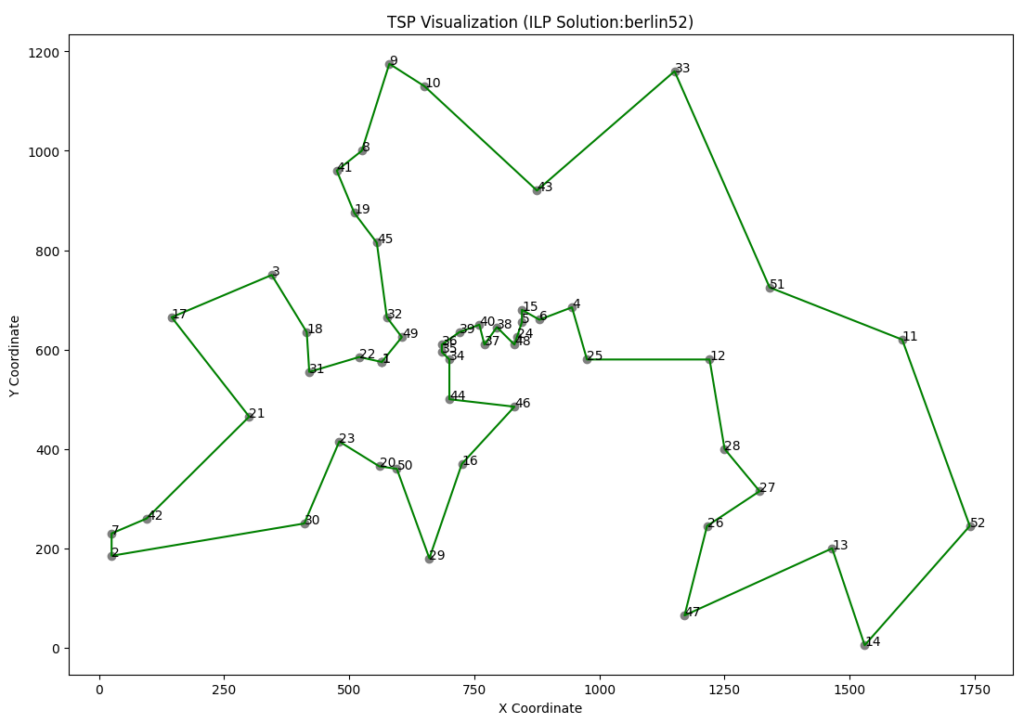
*Optimal solution of the berlin52 TSP instance with total distance 7544.365901904089 units.*

Using CP-SAT solver from Google OR-Tools, the berlin52 instance can be solved in 7 seconds (on an Intel(R) Core(TM) i7-8665U CPU @ 1.90GHz 2.11 GHz running Windows 10 Enterprise). On PC with the same hardware running Linux it would probably take half the time.